Detailed Description

A statistical filter for state likelihood estimation: the Kalman filter.

Author: Michael Reisecker

Date: 2019-07

Introduction
The Kalman filter : Overview, Algorithm, Example: Sensor fusion, Example: Vehicle entering a tunnel
Other features : Control signal input, Error estimation, Time-variant covariance matrices, Further notes
List of ini keys

Introduction

Note: After you have read this, some concepts are further explained in FilterParticle; references are also found there. The documentation is meant to be read in conjunction.; It is advised that you have a TeX installation in place to compile this part of the documentation yourself.

This filter suite implements a particle and a Kalman Filter.

Disclaimer: The Kalman and particle filters are not meant for operational use, rather they aim to be an accessible framework to scientific research backed by the convenience of MeteoIO, to quickly try a few things.

What do they do?

Both filters follow a statistical approach. The particle filter is a classical Monte Carlo method and samples states from a distribution function. The Kalman filter solves matrix equations of Bayesian statistics theory. They solve the problem of combining model data with noisy measurements in an optimal way.

Who are they for?

a) Suppose you have your toolchain set up with MeteoIO and are interested in Bayesian filters. With this software, you can (relatively) easily start to explore in this direction and hopefully decide if it is an idea worth pursuing.

b) You try a filter, play with the settings, and for whatever reason it works.

The difference to other, easier to use, filters is that you, the user, must provide the Physics in form of analytical models and covariance matrices. Almost all will be defaulted, but this may not make much sense in your use case.

The Kalman filter

A Kalman filter works on a linear state model which propagates an initial state forward in time. At each time step, the filter will adjust this model taking into account incoming measurements tainted with white (Gaussian) noise. For this, we can tune how much trust we put in our measurements (initial and online), and thus how strongly the filter will react to observations.

Note: In this scope, "online" means that new measurements can be incorporated on the fly as they come in without having to recalculate the past.

Overview

You need your linear model function in matrix form, initial values at \(T=0\) and a second model that relates observations to the internal states. If the model describes the measured parameters directly, this is the identity matrix. You supply an initial trust in the initial states, and this matrix will be propagated as error estimation. Furthermore, you assign a level of trust in the model function, and a level of trust in the measurements.

Algorithm

The Kalman filter solves the following set of recursive equations:

Prediction:

\[ \hat{x}_k=A\hat{x}_{k-1} + B u_k \]

\[ P_k = A P_{k-1}A^T+Q \]

Update:

\[ K_k = P_k H^T(H P_k H^T + R)^{-1} \]

\[ \hat{x}_k = \hat{x}_k + K_k(\hat{z}_k - H\hat{x}_k) \]

\[ P_k = (I - K_k H)P_k \]

where \(\hat{x}_k\) is the model value at time step \(k\), \(A\) is the model itself, i. e. the system transformation matrix, \(u_k\) is a control signal that is related to the states via \(B\), \(P\) is an error estimation, and \(Q\) is the covariance matrix of the process noise. Furthermore, \(\hat{z}_k\) is the observation at time step \(k\), \(K\) denotes the Kalman gain, \(H\) is the observation model relating observations to the states, \(R\) is the observation covariance matrix, and \(I\) is the identity. For details see Ref. [AM+02] equations (8)-(16).

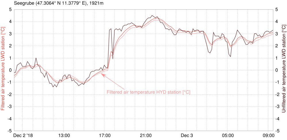
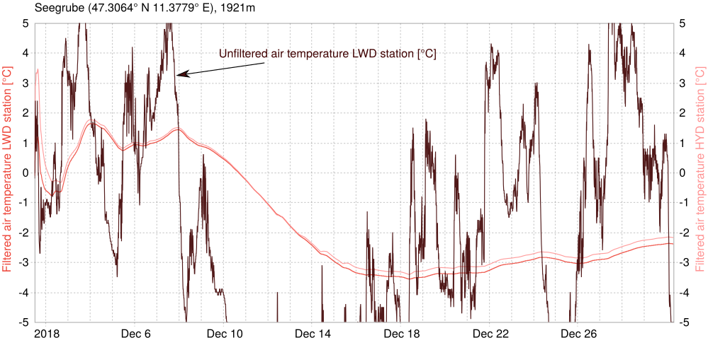
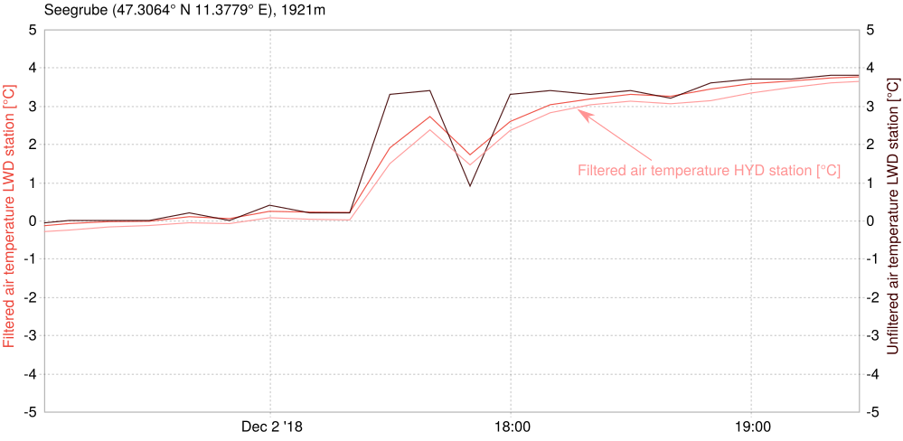
Note: These statistical methods stem mostly from robotics, where the state tracking is used to narrow down the position of a vehicle given noisy secondary measurements. In contrast, see for example Ref. [SC06] for an assessment of snow data assimilation through an (Ensemble) Kalman filter.

Example: Sensor fusion

Let's start with a real-world example and work through the settings.

Note: This example is exercised in the /doc/examples/statistical_filters.cc program to follow along.

At Innsbruck's Seegrube, there is a spot were two stations from different owners are situated right next to each other. Of course they both measure the air temperature and we want to use the Kalman filter to find the most likely real temperature.

Note: The Kalman filter can only be used for linear models (that can be expressed in matrix form). It is only valid for Gaussian measurement noise.

TA::FILTER1 = KALMAN

First, we need the heart of the problem, our system model. It describes the evolution of the states through time and is read from the STATE_DYNAMICS key. This is the matrix A from above. Matrices can be input in three different ways:

A scalar that the matrix diagonal is filled with.
A vector that is put on the diagonal.
A complete matrix. Matrices and vectors are input by a list of comma-separated elements. To init both a vector that is 4 elements long or a matrix that is 2 by 2 you would write: 1, 0, 0, 1. You can put brackets around your numbers for readability: [1, 0][0, 1].

We will use a most easy model:

STATE_DYNAMICS = 1

This means that we assume a constant temperature throughout our data window.

Note

You can use the following substitutions in the system matrix:

"dt" will be replaced with the normalized and scaled time delta between the current and the last measurement. At T=0, dt=0. At time of the first observation, dt=1.
"meteo(XX)" where "XX" stands for any meteo parameter present in the data set at this time, e. g. "meteo(TA)".

Next, we need an initial state. We have two internal states (both of which are energy states), namely the two temperatures. For both filters, you can provide the values as a list (e. g. 268, 271). You can also leave all of them or some of them empty to make MeteoIO pick the initial state(s) from the 1st available observation(s). "1st" is a synonym for this. You can use the token "average" (case sensitive) to let MeteoIO average over all 1st observations. We want the average between the first measurement of both stations so we write:

INITIAL_STATE = [average, average]

Note: Other valid input formats would be to not use this key (to pick earliest observation for all states) or [268, ] (to set the first state to 268 and pick the earliest measurement of the second observation variable for the 2nd state. Identical: [268, 1st]).; This is usually the line that fixes the number of states and thus the matrix sizes. MeteoIO will complain if they don't match, but input errors could still lead to surprising results.; MeteoIO will handle cases where the user requests to choose initial values automatically, but nodata values are encountered. It will search for the first valid dataset, and use this for the beginning of the measurement. If any one initial state encounters nodata values only, an error is thrown. If the filter itself encounters nodata values a warning is displayed. This makes it run but could have undesired side effects. As the number of nodata values increases, the results will become more and more skewed. A warning will be displayed; you should resample beforehand.

We have our states initialized and our state transition matrix ready. Now we need some statistical quantities. We provide the trust in the initial state via the INITIAL_TRUST key. This inputs the matrix P from above. Set low values if you don't trust \(\hat{x}_0\), and very high ones if you do. Let's not worry about it too much and pick a not very trusty 1 at the diagonal:

INITIAL_TRUST = 1

Note: Other valid input formats that do exactly the same would be [1, 0] [0, 1] (full matrix), [1, 1] (diagonal vector), or 1, 1 (you do not need brackets).

Next, we need the covariance of the process noise (noise in the model function by external forces acting on the state variables). A poor process model might be mitigated by injecting enough uncertainty here. We don't have knowledge of any specific process disturbances but we know that our model is quite crude, so we inject a bit of uncertainty in the model:

PROCESS_COVARIANCE = 0.05

Note: The above line will construct this 2x2-matrix: [0.05, 0][0, 0.05].

We now have everything regarding the system model. On to the observations.

The matrix \(H\) from above is the observation model relating our measurements to the internal states. In our case, we measure the temperatures which are also our internal states, so there is nothing to do. We can however decide how much each station contributes to the estimate. Let's trust both stations the same:

OBSERVATION_RELATION = [1, 1]

Next, the matrix \(R\) which is the observation covariance. Let's assume a standard deviation sigma of 0.8, i. e. the uncertainty of the sensor is somewhere around 0.8 °C and we put the variance (sigma squared) on the diagonal:

OBSERVATION_COVARIANCE = 0.64

Note: If \(Q\) and \(R\) are time invariant then \(P\) and \(K\) will stabilize quickly, cf. Fig. 5 (they could even be computed offline).

Only thing missing is a list of parameters that stand for the states. The filter runs on TA which is the first state, and we want the second one to be TA_HYD. By default, MeteoIO will only filter TA in the output file. This is to comply with all other filters and avoid unexpected results. We can set however that all observations that are filtered internally are also filtered in the meteo set:

ADD_OBSERVABLES = TA_HYD

FILTER_ALL_PARAMETERS = TRUE

Note that we require the number of observables to be equal to the number of states, simply to avoid having to set how many, and which, observables to output. You must supply them, but you can easily discard them (e. g. by leaving FILTER_ALL_PARAMETERS = FALSE or by designing your matrices in a way that they zero out).

Important: For technical reasons, filtering other parameters than the one the filter runs on only works as expected when the Kalman filter is the last filter that is applied!

Note: If you want to output all filtered parameters but also keep the originals you can simply use MeteoIO's COPY command.

The complete ini section now reads:

[FILTERS]
TA::FILTER1                          =   KALMAN
TA::ARG1::STATE_DYNAMICS             =   1
TA::ARG1::INITIAL_STATE              =   [average, average]
TA::ARG1::INITIAL_TRUST              =   1
TA::ARG1::PROCESS_COVARIANCE         =   0.05
TA::ARG1::ADD_OBSERVABLES            =   TA_HYD
TA::ARG1::FILTER_ALL_PARAMETERS      =   TRUE
TA::ARG1::OBSERVATION_RELATION       =   1
TA::ARG1::OBSERVATION_COVARIANCE     =   0.6

Fig. 1: Kalman filtering result with a process covariance of 0.05 and an observation covariance of 0.6, i. e. there is a little uncertainty injected in the system model and the observation is expected to be noisy with approximately sqrt(0.6) degrees uncertainty.

Fig. 2: Kalman filtering result with a process covariance of 0 and an observation covariance of 0.6, i. e. the model is trusted completely.

Fig. 3: Kalman filtering result with a process covariance of 0.2 and an observation covariance of 0.3, i. e. a middle ground where spikes are followed, but not to an extreme extent.

Example: Vehicle entering a tunnel

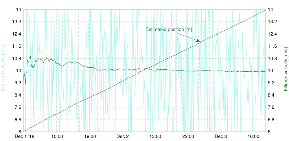
Let's tackle an accessible non-meteo standard problem for a Kalman filter to help understand the input mechanics better. Suppose a car enters a tunnel and can still reliably measure its speed, but not its position.

XX::FILTER1 = KALMAN

Note: The program in /doc/examples/statistical_filters.cc fakes noisy measurements of the velocity in x-direction (a constant true speed plus noise) and MeteoIO will read this in the SPEED parameter.

This is our model for the position and (constant) speed:

\[ x_t = x_{t-1} + \frac{\mathrm{d}x_{t-1}}{\mathrm{d}t} * dt \]

\[ \frac{\mathrm{d}x_t}{\mathrm{d}t} = \frac{\mathrm{d}x_{t-1}}{\mathrm{d}t} \]

Note: As mentioned earlier, in this implementation you need to provide observation fields for all states. Even if we do not measure either of the position coordinates fields must be created for them so that MeteoIO can output all (filtered) internal states. In this case they can be viewed as internal calculations and be discarded if we're only interested in the velocity.; Our car travels only in x-direction and \(v_y\) remains zero.

[INPUT]
XX::CREATE             =        CST
XX::CST::VALUE         =        0
YY::CREATE             =        CST
YY::CST::VALUE         =        0
VX::COPY               =        SPEED ;preserve original
VY::CREATE             =        CST
VY::CST::VALUE         =        0

We fix our state vector to be ordered [position in x, position in y, speed in x, speed in y]:

\[ \hat{x}=\left( \begin{array}{c} x \\ y \\ v_x \\ v_y \end{array} \right) \]

Therefore, the system model can be written in matrix form such that \(\hat{x}_t = A\hat{x}_{t-1}\):

\[ A=\left( \begin{array}{cccc} 1 & 0 & dt & 0 \\ 0 & 1 & 0 & dt \\ 0 & 0 & 1 & 0 \\ 0 & 0 & 0 & 1 \end{array} \right) \]

To select the measured velocities we design H to be:

\[ H=\left( \begin{array}{cccc} 0 & 0 & 0 & 0 \\ 0 & 0 & 0 & 0 \\ 0 & 0 & 1 & 0 \\ 0 & 0 & 0 & 1 \end{array} \right) \]

Keep in mind that we are only measuring the velocities, not the positions, so only the velocities can play a role in the new state estimation (Eq. 2 of update step). The initial values are position \((0, 0)\) and speed \((x_0, 0)\), and we pick the first measured speed as initial value:

STATE_DYNAMICS       = [1, 0, dt, 0][0, 1, 0, dt][0, 0, 1, 0][0, 0, 0, 1]
INITIAL_STATE        = [0, 0, 1st, 0]
OBSERVATION_RELATION = [0, 0, 0, 0][0, 0, 0, 0][0, 0, 1, 0][0, 0, 0, 1]

Note: Once again, in this case we could internally use 2 measurements only \((v_x, v_y)\); H could then be a 2x4-matrix, R could be a 2x2-matrix and the formulas would still work out. However, since all states are propagated anyway it is next to no penalty to work with square matrices and output them all.

With our states ordered the way they are the filter must run on x so that this is also internally the first observable. Then we match the rest of our vector ordering:

ADD_OBSERVABLES = YY VX VY

With some covariances (we have a perfect model now) and error output the whole ini section reads like so:

FILTER1                    =   KALMAN
STATE_DYNAMICS             =   [1, 0, dt, 0][0, 1, 0, dt][0, 0, 1, 0][0, 0, 0, 1]
INITIAL_STATE              =   [0, 0, 1st, 0]
INITIAL_TRUST              =   10
PROCESS_COVARIANCE         =   0
ADD_OBSERVABLES            =   YY VX VY
FILTER_ALL_PARAMETERS      =   TRUE
OBSERVATION_RELATION       =   [0, 0, 0, 0][0, 0, 0, 0][0, 0, 1, 0][0, 0, 0, 1]
OBSERVATION_COVARIANCE     =   10
OUT_ESTIMATED_ERROR        =   ERR1 ERR2 ERR3 ERR4
OUT_ERROR_AS_STDDEV        =   TRUE

Fig. 4: The measured velocity is all over the place, but the filtered one quickly stabilizes to the true speed (10 m/s). With a perfect model like this the secondary estimation of the position is almost linear like it should be.

Other features

Control signal input

With CONTROL_SIGNAL you can input an external control signal acting on the states (the vector \(\hat{u}\) from above) in three different ways:

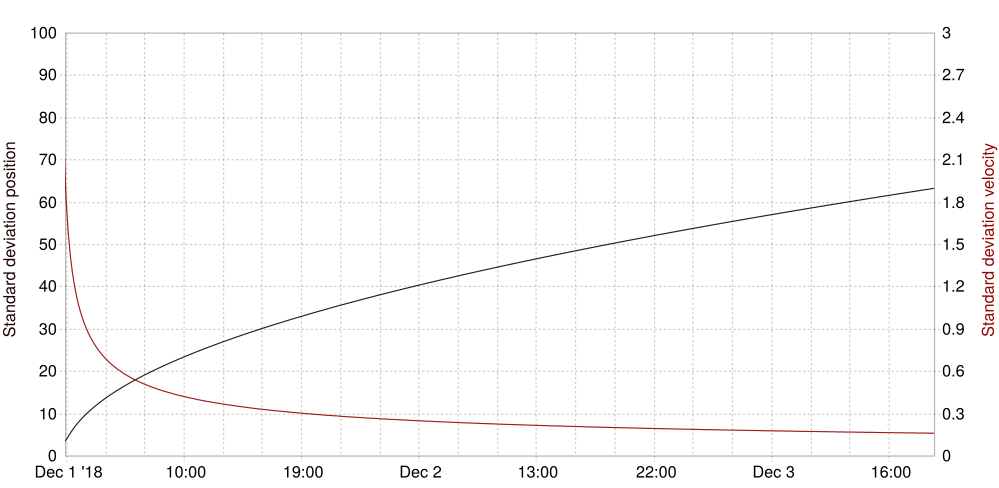
A scalar (e. g. 0.2) that an appropriate vector is filled with.
A vector (e. g. [0.1, 0.2]) which will be applied for all time steps.
A list of meteo parameters holding the value for each timestep (e. g. UU1 UU2), i. e. a time-variant vector. The matrix \(H\) is applied to this vector and can be input via CONTROL_RELATION as usual.

Error estimation

OUT_ESTIMATED_ERROR lets you pick one or more field names that the filter will output the evolution of the diagonal elements of the error estimation \(P\) to. Considering the diagonal elements to be variances you can also take the square root of this value for convenience with the OUT_ERROR_AS_STDDEV key.

OUT_ESTIMATED_ERROR = ERR1 ERR2 ;2 states

OUT_ERROR_AS_STDDEV = TRUE

If you have two states, you need two parameter names (that will be created).

Fig. 5: Diagonal components of the error estimation matrix from the velocity example: the estimated position becomes more and more unreliable, while with each new measurement the speed becomes more and more certain.

Time-variant covariance matrices

With PROCESS_COVARIANCE_PARAMS and OBSERVATION_COVARIANCE_PARAMS you can supply a list of parameters that \(Q\) and \(R\) are read from, i. e. time-variant covariance matrices. This has priority over a fixed matrix that is found in PROCESS_COVARIANCE and OBSERVATION_COVARIANCE, respectively. They can only be input as vectors that will be put on a matrix diagonal with the rest being 0. For this you need one meteo parameter per vector element (state) and you need to name the parameters with PROCESS_COVARIANCE_PARAMS and OBSERVATION_COVARIANCE_PARAMS.

PROCESS_COVARIANCE_PARAMS = COV_P1 COV_P2 //if either is missing, this key will be ignored

OBSERVATION_COVARIANCE_PARAMS = COV_O1 COV_O2

Suppression of warnings

The VERBOSE keyword can be used to enable/disable some warnings the filter shows in the console. This will normally concern missing input that was defaulted or something similar. Usually you will want to get rid of all of them, but if the filter must be quiet no matter what then you can set VERBOSE = FALSE.

Further notes

While matrices are input as comma-separated values, other lists are read from a space delimited line (e. g. PROCESS_COVARIANCE_PARAMS = COV1 COV2 COV3).
You may find MeteoIO's [DATASOURCEXXX] command to read multiple input files and stream them to the same container useful to combine meteo data and model input.
Important: For technical reasons all filters can run on a larger time frame than is requested in the getMeteoData call. This allows windowed filters to have enough data even at the beginning and end to do their work and is controlled by the BUFF_BEFORE and BUFFER_SIZE keys. If you set both to 0 then the filters receive exactly the time frame covered by the input dates. However, if you are using windowed filters also, then these will lack data. This is important in understanding how the initial states are picked: if MeteoIO inits the states automatically with the first available data point then this is taken from the first point MeteoIO sees. Thus, with a large enough buffer the model will start at a much earlier date and initial states are also picked a while before the input start date. Additionally, if there are nodata elements in there then even if they would be ignored for the output they would make the filters display warnings. You have to be careful to either start your analytical model at the date data window - buffer, or ideally provide exactly the same amount of data on the file system as you request MeteoIO to filter.

List of ini keys

Keyword	Meaning	Optional	Default Value
STATE_DYNAMICS	State transition matrix ( \(A\)).	no	-
INITIAL_STATE	State of the system at T=0 ( \(\hat{x}_0\)).	yes	empty, meaning 1st measurement will be picked
INITIAL_TRUST	Trust in the initial state ( \(P_0\)).	yes	1, meaning an appropriate identity matrix
PROCESS_COVARIANCE	Process noise covariance matrix (trust in the model, \(Q\)).	yes	0, meaning a matrix with all zeros
ADD_OBSERVABLES	List of observables in addition to the one the filter runs on.	yes	empty, meaning we have 1 state resp. 1 observable
FILTER_ALL_PARAMETERS	Filter only the parameter the filter runs on, or all states?	yes	FALSE, but TRUE is useful
OBSERVATION_RELATION	Linear model relating the observations to the states ( \(H\)).	yes	1, meaning identity matrix
OBSERVATION_COVARIANCE	Observation noise covariance matrix (trust in the measurements, \(R\)).	yes	0
CONTROL_SIGNAL	External control signal acting on the states ( \(\hat{u}\)).	yes	0
OUT_ESTIMATED_ERROR	Parameter name(s) to output error evolution to.	yes	empty
OUT_ERROR_AS_STDDEV	If TRUE, take the square root of error parameters.	yes	FALSE
PROCESS_COVARIANCE_PARAMS	List of parameter names to read \(Q\) from.	yes	empty
OBSERVATION_COVARIANCE_PARAMS	List of parameter names to read \(R\) from.	yes	empty
VERBOSE	Output warnings to the console.	yes	TRUE, warnings should be mitigated

Read on at FilterParticle.

#include <FilterKalman.h>

Public Member Functions
	FilterKalman (const std::vector< std::pair< std::string, std::string > > &vecArgs, const std::string &name, const Config &cfg)

virtual void	process (const unsigned int &param, const std::vector< MeteoData > &ivec, std::vector< MeteoData > &ovec)
	The filtering routine as called by the processing toolchain. More...

Public Member Functions inherited from mio::ProcessingBlock
virtual	~ProcessingBlock ()

virtual void	process (const unsigned int &param, const std::vector< MeteoData > &ivec, std::vector< MeteoData > &ovec)=0

virtual void	process (Date &dateStart, Date &dateEnd)

std::string	getName () const

const ProcessingProperties &	getProperties () const

const std::string	toString () const

bool	skipStation (const std::string &station_id) const
	Should the provided station be skipped in the processing? More...

bool	noStationsRestrictions () const

const std::vector< DateRange >	getTimeRestrictions () const

bool	skipHeight (const double &height) const
	Should the provided height be skipped in the processing? More...

Additional Inherited Members
Static Public Member Functions inherited from mio::ProcessingBlock
static void	readCorrections (const std::string &filter, const std::string &filename, std::vector< double > &X, std::vector< double > &Y)
	Read a data file structured as X Y value on each lines. More...

static void	readCorrections (const std::string &filter, const std::string &filename, std::vector< double > &X, std::vector< double > &Y1, std::vector< double > &Y2)
	Read a data file structured as X Y1 Y2 value on each lines. More...

static std::vector< double >	readCorrections (const std::string &filter, const std::string &filename, const size_t &col_idx, const char &c_type, const double &init)
	Read a correction file applicable to repeating time period. More...

static std::vector< offset_spec >	readCorrections (const std::string &filter, const std::string &filename, const double &TZ, const size_t &col_idx=2)
	Read a correction file, ie a file structured as timestamps followed by values on each lines. More...

static std::map< std::string, std::vector< DateRange > >	readDates (const std::string &filter, const std::string &filename, const double &TZ)
	Read a list of date ranges by stationIDs from a file. More...

Static Public Attributes inherited from mio::ProcessingBlock
static const double	default_height

Protected Member Functions inherited from mio::ProcessingBlock
	ProcessingBlock (const std::vector< std::pair< std::string, std::string > > &vecArgs, const std::string &name, const Config &cfg)
	protected constructor only to be called by children More...

Static Protected Member Functions inherited from mio::ProcessingBlock
static void	extract_dbl_vector (const unsigned int &param, const std::vector< MeteoData > &ivec, std::vector< double > &ovec)

static void	extract_dbl_vector (const unsigned int &param, const std::vector< const MeteoData * > &ivec, std::vector< double > &ovec)

Protected Attributes inherited from mio::ProcessingBlock
const std::set< std::string >	excluded_stations

const std::set< std::string >	kept_stations

const std::vector< DateRange >	time_restrictions

std::set< double >	included_heights

std::set< double >	excluded_heights

bool	all_heights

ProcessingProperties	properties

const std::string	block_name

Static Protected Attributes inherited from mio::ProcessingBlock
static const double	soil_albedo = .23

static const double	snow_albedo = .85

static const double	snow_thresh = .1
	parametrize the albedo from HS More...

Constructor & Destructor Documentation

◆ FilterKalman()

mio::FilterKalman::FilterKalman	(	const std::vector< std::pair< std::string, std::string > > &	vecArgs,
		const std::string &	name,
		const Config &	cfg
	)

Member Function Documentation

◆ process()

void mio::FilterKalman::process	(	const unsigned int &	param,
		const std::vector< MeteoData > &	ivec,
		std::vector< MeteoData > &	ovec
	)

virtual

The filtering routine as called by the processing toolchain.

Parameters

[in]	param	Parameter index the filter is asked to run on by the user.
[in]	ivec	Meteo data to filter.
[out]	ovec	Filtered meteo data. Cf. main documentation.

Implements mio::ProcessingBlock.

The documentation for this class was generated from the following files: