Detailed Description

A Monte Carlo sampling method: the particle filter.

Author: Michael Reisecker

Date: 2019-07

Introduction
The particle filter : Overview, Algorithm, Example: Mockup snow model, Example: Literature model function, Example: Gridded solar model input
Other features : Resampling, Final state estimation, Online state tracking, Seeding the random number generators
List of ini keys, Roadmap
Bibliography

Introduction

Note: Some concepts are explained beforehand in FilterKalman, you should read that first. The documentation is meant to be read in conjunction.; It is advised that you have a TeX installation in place to compile this part of the documentation yourself.

Disclaimer: These particle and Kalman filters are not meant for operational use, rather they aim to be an accessible framework to scientific research backed by the convenience of MeteoIO, to quickly try a few things.

The particle filter

This program implements a particle filter, also called a sequential Monte Carlo filter. Briefly, a particle filter propagates a state in state space by drawing from a proposed importance density and weights these particles according to the likelihood that the system is in a certain state taking into account noisy (!) measurements via Bayesian statistics.

Implemented is a SIR (Sampling Importance Resampling) algorithm, which is derived from the SIS (Sequential Importance Sampling) algorithm by

Choosing the prior as proposed importance density.
Resampling at every time step (although this can be tuned with a simple heuristic here).

(For a SIS algorithm, we would not use the prior pdf as importance density q, but rather choose one that is specific to the model. Then, the update formula for the weights becomes a little more complex, but the work is in actually choosing q. Such filters may be more robust against outliers.)

It operates in two stages: prediction and update based on new measurements coming in by applying a recursive Bayesian filter. This can be done online, which means that any new measurement can be augmented without having to recalculate the past. Although these are Monte Carlo simulations, they form a rigorous framework for state dynamics. With a large enough number of particles, the filter approximates the optimal solution to the problem of estimating the most likely state of a system taking into account all available information.

Physically speaking, we generate mass-energy-points (which, in our favor, can't change too rapidly due to their inertia) and place them in the state space. Mathematically, this is represented by delta-functions that are scaled by the prior probability density and summing over them yields the probability p, or rather, an approximation thereof. These particles are assigned a weight that is essentially (derived from) the Bayesian statistics formula \(P(A|B) = P(B|A) * P(A) / P(B)\) expressing a degree of belief in the estimated state.

Contrary to a Kalman filter (FilterKalman), a particle filter is able to emulate truly nonlinear model functions as well as arbitrary probability density functions.

The syntax follows Ref. [AM+02] and all remarks here can be investigated further therein.

INPUT:

Two models are required:

A model describing the evolution of the state with time (the system model).
A model relating the noisy measurements to the state (the measurement or observation model).

OUTPUT:

The likely posterior probability density function of the state based on all available information.

Overview

The particle filter needs a model function that describes the evolution of the states, and its starting values. Alternatively, you can pick a meteo parameter from your dataset that a curve is fitted against. You also need an analytical observation model to relate the measured observables to the internal states of the model function. If the model describes the measured parameter directly, then \(obx(x) = x\). Finally, the distributions for the model noise, observation noise, and prior distribution (for \(x_0\)) must be configured.

This implementation propagates a single state only, but you can obviously run the filter on each meteo parameter separately and you can also use every meteo parameter in the model. However, there is no way to update more than one state in the model equation itself (i. e. no vector maths).

Algorithm

The following algorithm is implemented (algorithm 4 of Ref. [AM+02]):

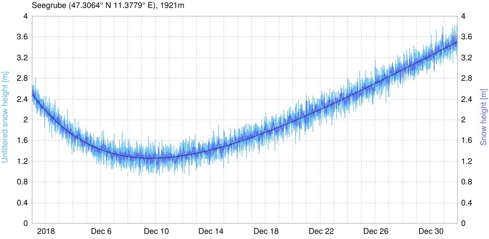
Set an initial state \(x_{0, 0}\). Add noise to this with the prior distribution to generate \(x_{0, 1...N}\) starting particles.
For each of the N particles at \(T=0\) compute the model function.
Add system noise to each particle with the model noise distribution.
Calculate the observation function of each particle and add noise with the observation noise distribution.
Calculate the likelihood of this noisy modeled observation given the real measurement via the observation distribution's probability density function.
Set weights for the particles connected to this likelihood ([AM+02] Eq. 63).
Resample the particle trajectories (algorithm 2 of Ref. [AM+02]).
Repeat 2-7 for each time step T.
Take the mean particle path (or the one with the highest weight) and calculate the observation function.

Note: Critique about these workings welcome here. The core parts in the code are prefaced with * PARTICLE FILTER * and * KALMAN FILTER * and shouldn't be too hard to read.

Example: Mockup snow model

Let's work through another example. Once more we fake an observation so we know the true process. If some snow melts in the first half of the month before it starts to snow again we could describe this with:

\[ x_k = x_{k-1} * a + b * u \]

With a and b being simple scalars and u being a factor that depends on the time step k. The program in /doc/examples/statistical_filters.cc will calculate this function for some preset \(x_0\), add system and observation noise to it, and write the simulated measurements to a file, as well as u. Within MeteoIO, we act as if this was a real measurement.

Note: Ref. [MG+14] is a great text to see these Bayesian methods be put to use for meteorological data. You will find a lot of useful information including a small snow model. [LM11] is written to similar ends. Both papers have a look at whether these statistical filters are viable for snow cover estimation and they compare different methods in basic research form.

HS::FILTER1 = PARTICLE

We enter the system model with the SYSTEM_MODEL key. The control signal u from above is saved into the meteo data as CTRL, so when MeteoIO runs it has it available as this parameter. The observation model is simply \(obs(x) = x\) again (cf. identity matrix in sensor fusion example) and we assume 2.5 m snow initially:

MODEL_FUNCTION     = x_km1 * 0.999 + 0.001 * meteo(CTRL)
OBS_MODEL_FUNCTION = xx
INITIAL_STATE      = 2.5

Fig. 1: Overview of the mockup snow model: The dark blue line is the true model function, light blue is with superimposed noise (twice actually - with system and observation noise), and the violet one is Kalman filtered.

Note

You can use the standard arithmetic operations, angular functions, exponentials, and some combinatorics which are parsed by tinyexpr. See here for a list of supported functions.

Additionally, the following substitutions are available for the system and observation models:

Current index (number of the time step): "kk"
Current time step: "tt"
Current state variable: "xx"
State at the previous time step: "x_km1" (read: \(x_{k-1}\))
Any available meteo parameter: "meteo(PARAM)"
Number 3 is only available for the observations model and number 4 picks the initial state for T=0 for the observation model.

The time vector tt is a normalized and shifted version of the date such that the time of the first measurement is at 0 and the second one is at 1. Suppose you had measurements at 00:00, 01:00, and 01:30 then kk would be [0, 1, 2] and tt would be [0, 1, 1.5].

At last, we set up our random number generators:

MODEL_RNG_DISTRIBUTION = GAUSS
MODEL_RNG_PARAMETERS   = 0 0.1 ;mean sigma
OBS_RNG_DISTRIBUTION   = GAUSS
OBS_RNG_PARAMETERS     = 0 0.3

Note: If the process noise is zero, then the particle filter is not appropriate as it is a method of estimating dynamic states.; Since we are not setting a different prior distribution via PRIOR_RNG_DISTRIBUTION and PRIOR_RNG_PARAMETERS we can omit these keys and the prior distribution will be chosen to be the model distribution. Same would be true for the observation distribution, but that one is slightly different here.; Read more about the random number generator settings here: RandomNumberGenerator.

Together, our ini file looks like this:

HS::FILTER1                          =   PARTICLE
HS::ARG1::MODEL_FUNCTION             =   x_km1 * 0.999 + 0.001 * meteo(CTRL)
HS::ARG1::OBS_MODEL_FUNCTION         =   xx
HS::ARG1::INITIAL_STATE              =   2.5
HS::ARG1::MODEL_RNG_DISTRIBUTION     =   GAUSS
HS::ARG1::MODEL_RNG_PARAMETERS       =   0 0.1
HS::ARG1::OBS_RNG_DISTRIBUTION       =   GAUSS
HS::ARG1::OBS_RNG_PARAMETERS         =   0 0.3

Fig. 2: Particle filtering on a mockup snow model. The distribution choices will greatly influence the result and can completely destroy the simulation.

Note: Neither of the two features separating the particle from the Kalman filter was actually used in this example. First, the noise was Gaussian again (cf. central limit theorem). Cumulative distribution functions are relatively hard to write, and only Gauss is implemented so far. If you need a specific one, you can request one here. Maybe at this time C99's gamma functions will be available. Secondly, the model function was linear again. The next example uses a nonlinear one.

Example: Literature model function

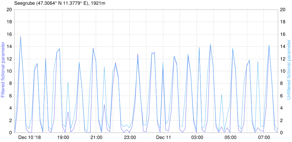
The following example function has nothing to do with meteo data, but it has been analyzed a lot in literature (e. g. in Ref. [AM+02] and Ref. [CPS92]) and it's nonlinear.

We change the functions and RNG parameters in the control program statistical_filters.cc:

RNGU.setDistributionParameter("mean", 0);
RNGU.setDistributionParameter("sigma", 3.3);
RNGU.setDistributionParameter("mean", 0);
RNGU.setDistributionParameter("sigma", 1);
...
xx = xx / 2. + 25. * xx / (1. + xx*xx) + 8. * cos(1.2 * kk);
const double obs = (xx + rr) * (xx + rr) / 20. + RNGV.doub();

Of course, we have to adapt our ini settings accordingly:

HS::ARG1::MODEL_FUNCTION             =   x_km1 / 2 + 25 * x_km1 / (1 + x_km1*x_km1) + 8 * cos(1.2 * kk)
HS::ARG1::OBS_MODEL_FUNCTION         =   xx*xx / 20
HS::ARG1::INITIAL_STATE              =   0
HS::ARG1::MODEL_RNG_DISTRIBUTION     =   GAUSS
HS::ARG1::MODEL_RNG_PARAMETERS       =   0 3.3
HS::ARG1::OBS_RNG_DISTRIBUTION       =   GAUSS
HS::ARG1::OBS_RNG_PARAMETERS         =   0 1

Fig. 3: Result of particle filtering a nonlinear function from literature. Also, the observation model is not trivial and we do not see a direct presentation of it which makes it harder to tell which spikes are 'real'.

Example: Gridded solar model input

For a particle filter, as well as for a Kalman filter, you absolutely need a model function. However, often you will only have data points that your or somebody else's model spits out. For this reason the particle filter allows you to fit a curve against the data points and use that as model function. The following fits are available: Fit1D, and the polynomial fit takes a 2nd argument with the degree of interpolation (default: 3).

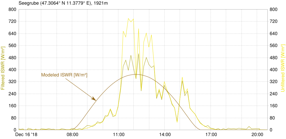
Let's use a MeteoIO internal model for the global radiation:

[InputEditing]

ISWR_MODEL::CREATE = CLEARSKY_SW ;depends on TA, RH

Comparing the values created this way with the measurements we can see that there is up to a couple of hundret W/m^2 difference between the two. This gap needs to be covered by the standard deviations of the random number generators. If you put small numbers here then the huge difference will be so unlikely that everything is filtered (as it should, because obviously it is not justified to put complete trust in this model). For example, if we say that the standard deviation for the measurement sensor is 30, and some of the discrepancy remaining is covered by a standard deviation of 100 in the model then the highest peaks are still deemed unlikely while the rest stays pretty much the same.

Using a little more particles our ini section reads:

ISWR::FILTER1                        =   PARTICLE
ISWR::ARG1::NO_OF_PARTICLES          =   1000
ISWR::ARG1::MODEL_FUNCTION           =   FIT POLYNOMIAL 5
ISWR::ARG1::MODEL_FIT_PARAM          =   ISWR_MODEL
ISWR::ARG1::OBS_MODEL_FUNCTION       =   xx
ISWR::ARG1::MODEL_RNG_DISTRIBUTION   =   GAUSS
ISWR::ARG1::MODEL_RNG_PARAMETERS     =   0 100
ISWR::ARG1::OBS_RNG_DISTRIBUTION     =   GAUSS
ISWR::ARG1::OBS_RNG_PARAMETERS       =   0 30

Fig. 4: A 5th degree polynomial fit is now the model function of the particle filter. Assigning different standard deviations to the model and measurements will greatly influence the results.

Other features

Resampling

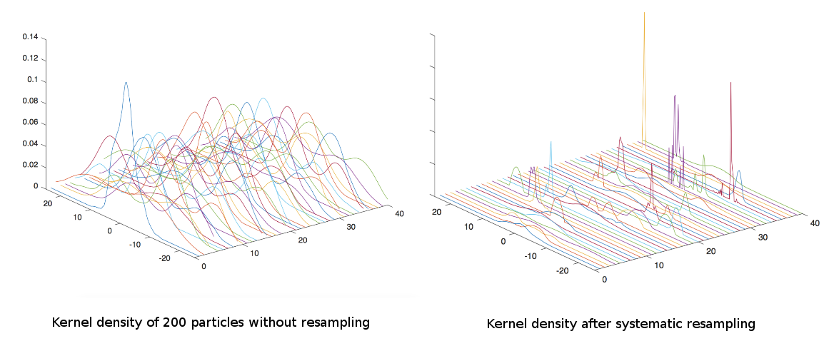
Resampling of the particle paths is turned on and off with the PATH_RESAMPLING key. If resampling is turned off then a lot of computational power may be devoted to particles with low weights that do not contribute significantly to the end result, and the paths may lose track of the main line. Usually, it is needed.

The RESAMPLE_PERCENTILE \(r_p\) lets you pick a factor to decide whether to resample: if \(N_{eff} < r_p * N\) then resample, where N is the number of particles and \(N_{eff}\) the effective sample size, [AM+02] Eq. 50. Strictly, a SIR algorithm requires resampling at each time step, but in practice a heuristic like this is appropriate (e. g. Ref. [DJ09]).

For now, only one resampling strategy is implemented:

SYSTEMATIC: Straight-forward systematic resampling. This helps avoid degeneracy by skipping particles with small weights in favor of more meaningful ones (algorithm 2 of Ref. [AM+02]). However, it does decrease diversity (by selecting particles with high weight multiple times) and for very small process noise the particles collapse to a single point within a couple of iterations ("sample impoverishment").

Note: Bruteforcing the particle number helps with the degeneracy problem.

Fig. 5: Kernel densities of the particles before and after resampling for the literature function example.

Note: The minimalistic MATLAB code used for this plot can be found as a comment in the /doc/examples/statistical_filters.cc program.

Final state estimation

In the end, the particle filter will estimate the most likely observation by taking the mean of all particles (sum of particles multiplied with their weight) and use that as input for the observation model. This is only one possible measure however and a second one is offered: at each time step, the particle with the highest weight is the observation model input:

ESTIMATION_MEASURE = MAX_WEIGHT

Online state tracking

The basics are there to aggregate new information online, i. e. to keep the state of the filter and simply apply any number of new measurements to it without recalculating the past. Although it may make sense to formulate models that take into account earlier time steps, often the added complexity outweighs the benefits. Hence, if each time step is calculated from only the previous state then it is enough to save the last state (particles and their weights) and resume from there.

Note: So far, a similar mechanism is lacking for the Kalman filter, but if needed / wanted it will be done if there's time.

DUMP_INTERNAL_STATES_FILE = ./output/particle_states.dat

INPUT_INTERNAL_STATES_FILE = ./output/particle_states.dat

If the input file is not found the filter will silently start with the initial states that are set through the ini file. In the example above the filter will not find an input file for the first run and thus use the initial states. In the end it writes the states to a file. The next time the filter is started the input file will exist and the calculation is resumed at this point. However, as of yet the model parameters (like kk, tt, ...) are not saved and that has to be taken into account for the analytical model output. If this would be needed / wanted, it will be built in. Be aware though that Ref. [DJ09] mentions that the number of time steps should not be too high per run.

You can also output the particles' paths as a big matrix:

DUMP_PARTICLES_FILE = ./output/particles.dat

Note: This is the input for Fig. 5.

Seeding the random number generators

You can seed all random number generators for reproducibility. To do this, set the appropriate keys as follows:

MODEL_RNG_SEED    = 89023457862 347891329870 6712368354 234890234 ;4 for XOR generator
PRIOR_RNG_SEED    = ...
OBS_RNG_SEED      = ...
RESAMPLE_RNG_SEED = ...

Note: The last one is an internal uniform generator needed by the particle filter itself (with fixed distribution parameters).; The number of seeds must match the one the RNG algorithm expects: cf. RandomNumberGenerator.

List of ini keys

Keyword	Meaning	Optional	Default Value
MODEL_FUNCTION	State transition function.	no, but can also be a fit	empty
MODEL_FIT_PARAM	Parameter in meteo set to fit model curve against.	yes, if MODEL_FUNCTION is set	empty
INITIAL_STATE	State variable at T=0.	yes	1st observation
OBS_MODEL_FUNCTION	Model relating the observations to the states.	yes, but you need one	"xx"
ESTIMATION_MEASURE	Which measure to use for the final estimation.	yes	MEAN (choices: MAX_WEIGHT)
NO_OF_PARTICLES	Number of particles per time step.	yes	500
PATH_RESAMPLING	Perform particle path resampling?	yes	TRUE, this is normally needed
RESAMPLE_PERCENTILE	Scalar for simple resampling heuristic.	yes	0.5
DUMP_PARTICLES_FILE	Output file path for the particles.	yes	empty
DUMP_INTERNAL_STATES_FILE	Output file path for the internal states.	yes	empty
INPUT_INTERNAL_STATES_FILE	Input file path for the internal states.	yes	empty
VERBOSE	Output warnings to the console.	yes	TRUE, warnings should be mitigated
MODEL_RNG_ALGORITHM	Random numbers generator function for the model.	yes	XOR
MODEL_RNG_DISTRIBUTION	Random numbers distribution for the model.	yes	GAUSS
MODEL_RNG_PARAMETERS	Random numbers distribution parameters for the model.	yes, but the filter is sensitive to them	RNG defaults
MODEL_RNG_SEED	Random numbers generator seed for the model.	yes	hardware seed
PRIOR_RNG_ALGORITHM	Random numbers generator function for the prior distribution.	yes	XOR
PRIOR_RNG_DISTRIBUTION	Random numbers distribution for the prior.	yes	GAUSS
PRIOR_RNG_PARAMETERS	Random numbers distribution parameters for the prior.	yes	RNG defaults
PRIOR_RNG_SEED	Random numbers generator seed for the prior.	yes	hardware seed
OBS_RNG_ALGORITHM	Random numbers generator function for the observations.	yes	XOR
OBS_RNG_DISTRIBUTION	Random numbers distribution for the observations.	yes	GAUSS
OBS_RNG_PARAMETERS	Random numbers distribution parameters for the observations.	yes	RNG defaults
OBS_RNG_SEED	Random numbers generator seed for the observations.	yes	hardware seed
RESAMPLE_RNG_SEED	Random numbers generator seed for the resampling.	yes	hardware seed

Roadmap

An interesting development would be to slowly follow Ref. [MG+14] to reach similar results, but generalized to arbitrary data and terrain. For this, spatially correlated random numbers are necessary and we would move towards gridded filters and spatial interpolations.

See Ref. [DJ09] for smoothing algorithms of this class that would run through the data forwards and backwards and have knowledge of all measurements, i. e. no live filtering.

Bibliography

[AM+02] M. Sanjeev Arulampalam, Simon Maskell, Neil Gordon, and Tim Clapp. A Tutorial on Particle Filters for Online Nonlinear/Non-Gaussian Bayesian Tracking. IEEE Transactions on Signal Processing, Vol. 50, No. 2, February 2002.
[CPS92] Bradley P. Carlin, Nicholas G. Polson, and David S. Stoffer. A Monte Carlo Approach to Nonnormal and Nonlinear State-Space Modeling. Journal of the American Statistical Association, Vol. 87, issue 418, 493-500, 1992.
[DJ09] Arnaoud Doucet and Adam M. Johansen. A Tutorial on Particle Filtering and Smoothing: Fifteen years later. Handbook of Nonlinear Filtering, Vol. 12, 2009.
[LM11] Marc Leisenring and Hamid Moradkhani. Snow water equivalent prediction using Bayesian data assimilation methods. Stoch Environ Res Risk Assess 25, 253-270, 2011.
[MG+14] Jan Magnusson, David Gustafsson, Fabia Hüsler, and Tobias Jonas. Assimilation of point SWE data into a distributed snow cover model comparing two contrasting methods. Water Resources Research, 50, 7816-7835, 2014.
[SC06] Andrew G. Slater and Martyn P. Clark. Snow Data Assimilation via an Ensemble Kalman Filter. Journal of Hydrometeorology, Vol. 7, 478ff., 2006.

#include <FilterParticle.h>

Public Member Functions
	FilterParticle (const std::vector< std::pair< std::string, std::string > > &vecArgs, const std::string &name, const Config &cfg)

virtual void	process (const unsigned int &param, const std::vector< MeteoData > &ivec, std::vector< MeteoData > &ovec)
	The filtering routine as called by the processing toolchain. More...

Public Member Functions inherited from mio::ProcessingBlock
virtual	~ProcessingBlock ()

virtual void	process (const unsigned int &param, const std::vector< MeteoData > &ivec, std::vector< MeteoData > &ovec)=0

virtual void	process (Date &dateStart, Date &dateEnd)

std::string	getName () const

const ProcessingProperties &	getProperties () const

const std::string	toString () const

bool	skipStation (const std::string &station_id) const
	Should the provided station be skipped in the processing? More...

bool	noStationsRestrictions () const

const std::vector< DateRange >	getTimeRestrictions () const

bool	skipHeight (const double &height) const
	Should the provided height be skipped in the processing? More...

Additional Inherited Members
Static Public Member Functions inherited from mio::ProcessingBlock
static void	readCorrections (const std::string &filter, const std::string &filename, std::vector< double > &X, std::vector< double > &Y)
	Read a data file structured as X Y value on each lines. More...

static void	readCorrections (const std::string &filter, const std::string &filename, std::vector< double > &X, std::vector< double > &Y1, std::vector< double > &Y2)
	Read a data file structured as X Y1 Y2 value on each lines. More...

static std::vector< double >	readCorrections (const std::string &filter, const std::string &filename, const size_t &col_idx, const char &c_type, const double &init)
	Read a correction file applicable to repeating time period. More...

static std::vector< offset_spec >	readCorrections (const std::string &filter, const std::string &filename, const double &TZ, const size_t &col_idx=2)
	Read a correction file, ie a file structured as timestamps followed by values on each lines. More...

static std::map< std::string, std::vector< DateRange > >	readDates (const std::string &filter, const std::string &filename, const double &TZ)
	Read a list of date ranges by stationIDs from a file. More...

Static Public Attributes inherited from mio::ProcessingBlock
static const double	default_height

Protected Member Functions inherited from mio::ProcessingBlock
	ProcessingBlock (const std::vector< std::pair< std::string, std::string > > &vecArgs, const std::string &name, const Config &cfg)
	protected constructor only to be called by children More...

Static Protected Member Functions inherited from mio::ProcessingBlock
static void	extract_dbl_vector (const unsigned int &param, const std::vector< MeteoData > &ivec, std::vector< double > &ovec)

static void	extract_dbl_vector (const unsigned int &param, const std::vector< const MeteoData * > &ivec, std::vector< double > &ovec)

Protected Attributes inherited from mio::ProcessingBlock
const std::set< std::string >	excluded_stations

const std::set< std::string >	kept_stations

const std::vector< DateRange >	time_restrictions

std::set< double >	included_heights

std::set< double >	excluded_heights

bool	all_heights

ProcessingProperties	properties

const std::string	block_name

Static Protected Attributes inherited from mio::ProcessingBlock
static const double	soil_albedo = .23

static const double	snow_albedo = .85

static const double	snow_thresh = .1
	parametrize the albedo from HS More...

Constructor & Destructor Documentation

◆ FilterParticle()

mio::FilterParticle::FilterParticle	(	const std::vector< std::pair< std::string, std::string > > &	vecArgs,
		const std::string &	name,
		const Config &	cfg
	)

Member Function Documentation

◆ process()

void mio::FilterParticle::process	(	const unsigned int &	param,
		const std::vector< MeteoData > &	ivec,
		std::vector< MeteoData > &	ovec
	)

virtual

The filtering routine as called by the processing toolchain.

Parameters

[in]	param	Parameter index the filter is asked to run on by the user.
[in]	ivec	Meteo data to filter.
[out]	ovec	Filtered meteo data. Cf. main documentation.

Implements mio::ProcessingBlock.

The documentation for this class was generated from the following files: